36 Path Analysis and SEM
36.1 Introduction
Path Analysis and Structural Equation Modelling (SEM) are advanced techniques that are used to examine the relationships that exist between different variables and to build models of these relationships.
They incorporate elements of other techniques that we have already covered, primarily regression, multiple regression, and factor analysis.
We’ll therefore begin by revising these techniques, before moving onto the focus of this section. Note that we are focusing on developing a conceptual understanding of the techniques, and will deal with their practical application in the following in-class practical.
Please remember that the purpose of this module is to introduce you to some of these advanced statistical techniques, and for you to gain a basic familiarity with them.
There is a lot more to these techniques than is covered here, and if you’re interested in them (for example, for use in your dissertation or on placement) it would definitely be worth exploring them further.
Regression
In regression analysis, we examine the relationship between a dependent variable and one or more independent variables.
The simplest form is called simple linear regression, which involves one independent variable (IV, or the ‘predictor’ variable) and one dependent variable (DV, or the ‘outcome’ variable).
![]()
- For example, we might examine whether
athlete age(IV) is a significant predictor ofoverall performance(DV) in an athletic competition.
In regression, we try to model the expected value of the DV based on the known values of the IV, allowing for prediction, forecasting, and understanding causal relationships.
- For example, if we know an athlete’s age, can we confidently predict their overall performance?
Multiple Regression
Multiple regression is an extension of simple linear regression. It’s designed to analyse the relationship between one dependent variable (DV) and several independent variables (IVs).
![]()
- For example, we might examine whether
athlete age,years of trainingandprevious performance(IVs) are significant predictors ofoverall performancein an athletic competition (DV).
It allows for the examination of how multiple predictors collectively influence the outcome variable.
It’s invaluable for ‘disentangling’ the individual effect of each IV while controlling for the influence of other IVs, providing a more comprehensive understanding of complex relationships.
For example, you may expect that age and years of training are not only significant predictors of performance, but are also associated with each other.
Factor Analysis
Factor Analysis was also covered in a previous section. It’s used to identify underlying variables, or factors, that explain the pattern of correlations within a set of observed variables.
![]()
- For example, we might assume that a set of variables such as
speed,power, andenduranceall represent an ‘underlying’ factor that could be called ‘fitness’, or ‘athleticism’.
We’d assume that someone who scores highly on one is more likely to score highly on another, because they are different dimensions of same factor. These are called ‘latent’ factors.
The idea of ‘general intelligence’ is based on the understanding that performance on different aspects of intelligence tests, such as mathematical calculation and logical reasoning, is influenced by an underlying factor that we can call ‘intelligence’.
Remember that the latent factor or factors are constructs that we cannot directly observe.
Factor analysis simplifies data interpretation by reducing the number of variables and revealing the underlying structure, helping in the development of more focused and interpretable models.
36.2 What is Path Analysis?
Introduction
Path Analysis is basically a specialised form of regression analysis. It allows us to visualise the direct and indirect relationships between variables in our data through developing a model of those relationships.
Imagine it as a map that shows how different factors in your data influence each other. Indeed, this is usually how a Path Analysis is presented.
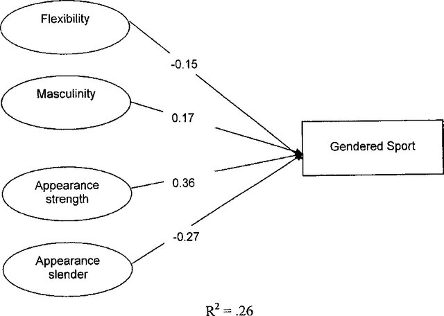
Here’s an example of a simple path analysis from a 2005 paper.
You can see that the authors have constructed a model that attempts to measure the influence of four independent variables (on the left) on a dependent variable (on the right).
The path analysis gives a really clear summary of the strength of the relationships they found, and their direction (positive or negative). The R2 figure at the bottom indicates the overall power of the model in explaining the variance within the dependent variable (basically, how ‘good’ is the model’?)
Key Concepts
Three concepts are central to Path Analysis.
![]()
The first is directionality. Path Analysis helps in understanding the direction of relationships between variables. The model above was a very basic example of such an analysis. However, they can become much more complex, as in the following example (from here).
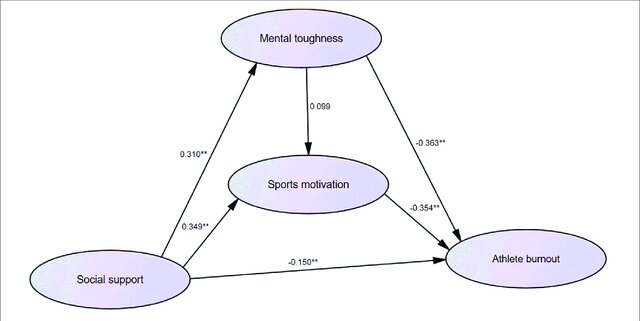
Note that in this path analysis, the researchers have created a model that examines (and visualises) relationships between a number of variables, and reinforces their argument that their independent variable (Athlete burnout) is influenced by three dependent variables that are in turn influenced by each other.
The second is hypothesis testing. Path Analysis is a hypothesis-driven approach. We start with a theory (usually that there are certain relationships between variables) and then test it using statistical data.
The third, as you’ve seen, is diagrammatic representation. Path diagrams are used to represent these relationships, making it easier to understand complex models. This is one of the key strengths of Path Analysis; it is relatively easy to present and explain in contrast to tables or other text-based outputs.
Mediating Variables
It’s important to understand the concept of ‘mediating variables’ in path analysis, and in quantitative research more generally.
Mediating variables are variables that explain the relationship between two other variables, typically an independent variable (IV) and a dependent variable (DV).
![]()
In a simple causal chain, the independent variable influences the mediating variable, which in turn affects the dependent variable. This mediation process is crucial for understanding how and why specific effects occur.
For example, in a study exploring the impact of education (IV) on income (DV), job opportunities could serve as a mediating variable, illustrating how education leads to better job prospects, which then results in higher income.
The significance of mediating variables lies in their ability to provide insight into the underlying mechanisms and processes that drive relationships between variables. This understanding is vital for both theoretical development and practical applications.
By identifying and testing these mediators, we can better understand the complexity of causal relationships, potentially revealing indirect effects that are not immediately apparent.
![]()
For instance, in health psychology, understanding how stress (IV) affects health (DV) may require exploring mediators like coping strategies,social support, and secure housing.
In statistical terms, mediating variables are assessed through a series of regression analyses that evaluate the paths between the independent, mediating, and dependent variables. The significance of these paths is determined through specific statistical tests like the Sobel test, which can ascertain whether the mediating effect is statistically significant.
This testing allows us to validate the mediation model, ensuring that the relationships are not spurious and that the mediating variable genuinely connects the independent and dependent variables.
Conducting a Path Analysis
![]()
First, we define our model. This involves identifying the variables that we’re interested in.
These will be independent variables (predictors), dependent variables (outcomes), and mediating or intervening variables (which mediate the relationship between predictors and outcomes).
Second, we specify our model in R. This ‘hands over’ the calculations to a package (such as lavaan), which will set up a series of regression equations.
So if we have a model where X influences Y, and Y influences Z, the equations that the package would use might look like this:
Equation for Y: \(Y = aX + e1\)
Equation for Z: \(Z = bY + e2\)
Here, \(a\) and \(b\) are path coefficients (like regression coefficients), and \(e1\) and \(e2\) are error terms.
In the third step, the package estimates the path coefficients (a, b, etc.). These coefficients tell us the strength and direction of the relationship between variables.
This is typically done by performing regression analysis and calculates the coefficients based on the least squares method, which minimises the sum of the squares of the errors (the differences between observed and predicted values).
The least squares method was covered earlier in this module.
Fourth, when we have our coefficients, we need to evaluate how well our model fits the data. This usually involves several statistics that are output by the package:
Chi-Square Test: A low chi-square value suggests a good fit. However, it’s sensitive to sample size.
Root Mean Square Error of Approximation (RMSEA): Values less than 0.05 indicate a good fit.
Comparative Fit Index (CFI): Values closer to 1 indicate a better fit.
Standardized Root Mean Square Residual (SRMR): Values less than 0.08 are generally considered good.
Finally, we can interpret the results. We’re interested in several things, including:
Direct, Indirect, and Total Effects: Direct effects are the influence of one variable directly on another. Indirect effects are influences that are mediated through one or more other variables. Total effects are the sum of direct and indirect effects.
Significance Testing: We can test if our path coefficients are statistically significant, typically using t-tests.
At this point, we’d also want to produce a visual representation of our model, making it easy to report and share with others.
36.3 Structural Equation Modelling (SEM)
SEM is a bit like Path Analysis, but more advanced. It combines factor analysis and multiple regression analysis, allowing us to examine a series of dependence relationships within our data simultaneously.
Key Concepts
Latent Variables
As noted above, ‘latent Variables’ are variables that are not directly observed but are inferred from other variables (like ’fitness’ or ‘athleticism’). They are similar to the ‘factors’ that we learned about in Factor Analysis. So they are theoretical constructs that are not directly observed, but are inferred from multiple observed variables.
These variables often represent abstract concepts like intelligence, satisfaction, or attitude. In SEM, latent variables help in explaining correlations between observed variables, providing a more nuanced understanding of the underlying constructs that drive the observable data.
They serve as the ‘backbone’ for hypothesis testing in SEM: we can create complex models involving multiple latent and observed variables and then statistically examine these models to understand relationships and causal paths within our data.
Model Fit
Just as in Path Analysis, in SEM we create a model that we ‘think’ will explain our data, and then examine how well that proposed model fits the data. Good fit = good model, bad fit = bad model. This lets us compare different models to see which is the ‘best’.
Example
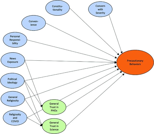
In the following SEM based on a Covid-19 study, the researchers have collected data on the independent variables (in blue).
They are interested in the association between these variables and their dependent variable (taking precautionary behaviours).
They have also hypothesised that there are two latent variables, in green.
Why do we use SEM?
SEM is ideal for studying complex relationships that are too intricate for standard regression models. This is particularly true where we think there are important underlying factors that haven’t been captured directly, or where we think there are important relationships between the variables in our data.
36.4 What’s the Difference?
It’s important to understand the distinction between Path Analysis and SEM, which are really two versions of the same thing.
The main difference lies in SEM’s ability to incorporate latent (unobserved) variables. While Path Analysis is limited to observed variables and direct relationships between IVs, mediating variables and a DV, SEM can model both observed and latent variables and can handle more complex causal structures between those variables.
Imagine you’re looking at a map of various roads and pathways between different landmarks. Path analysis is like tracing specific routes on this map to see how they directly connect. It focuses on the direct relationships between observable things (like how studying affects grades).
SEM, on the other hand, is like adding another layer to this map, with hidden tunnels and secret passages (latent variables) that you can’t see but know are there. It not only looks at the direct paths but also considers these ‘hidden’ factors (like motivation or stress) that might influence the journey, but aren’t directly visible.
So, while path analysis shows you the clear, direct routes, SEM gives you a deeper exploration of the map, including the hidden connections that influence the journey.
36.5 Reading
The following is an accessible introduction to SEM. It’s available via the module reading list on myplace:
- Schumacker, R. E. (2010). A beginner’s guide to structural equation modeling [internet resource] (R. G. Lomax, Ed.; 3rd ed..). Routledge.